In this tutorial, we're going to show you three ways to find the difference between two columns in Google Sheets. Each method can be used for slightly different applications so if the first one doesn't work for you take a look at the next one. If you would like to follow along here is the example worksheet.
Three Methods for Calculating Differences in Google Sheets
To find the difference between two columns in Google Sheets, you can use three techniques:
- Simple Formulas: Subtract one column from the other using a basic formula like "=A1-B1."
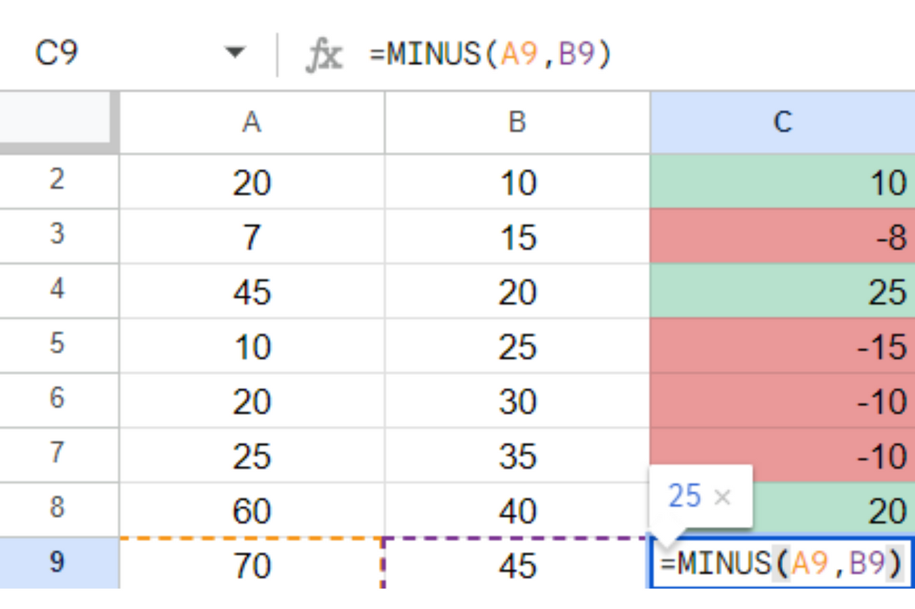
- "MINUS" Function: Utilize the built-in "MINUS" function by typing "=MINUS(A1, B1)" for each corresponding cell.
- Conditional Formatting: Highlight the differences visually by setting up conditional formatting rules for the third column based on whether the value is greater or less than zero.
Method 1: Using Simple Formulas
When we can keep things simple in Google Sheets it's often best to do so. simple formulas will allow others to quickly understand what is going on in the spreadsheet. In this method, we'll use a simple formula to calculate the differences between two columns.

- Create a Third Column: Click on a new column where you want the differences to appear. For example, if you have data in columns A and B, you can put the differences in column C.
- Input the Formula: In the first cell of the third column (C1), type the formula "=A1-B1". This formula calculates the difference by subtracting the value in cell B1 from that in cell A1.
- Auto-fill the Formula: After entering the formula in C1, click on the small blue circle at the bottom right corner of the cell (the fill handle) and drag it down to apply the formula to the entire column. Google Sheets will automatically adjust the cell references for each row.
Voilà! Column C will now show the differences between your two original columns. If you see a positive number in Column C, it means that the value in Column A is greater. Conversely, if it's negative, Column B is greater.
Method 2: Using the "MINUS" Function
Google Sheets also provides a built-in function for finding the difference between two values – the "MINUS" function. Here's how to use it:

- Create a Third Column: As before, click on a new column (e.g., column C) where you want the differences to appear.
- Input the Formula: In the first cell of the third column (C1), type "=MINUS(A1, B1)". This function subtracts the value in cell B1 from the value in cell A1.
- Auto-fill the Formula: Use the fill handle to drag the formula down the column, just like in Method 1.
Method 3: Using Conditional Formatting
If you want a more visual representation of the differences between two columns, you can use conditional formatting. Here we are going to combine the MINUS function with conditional formatting.
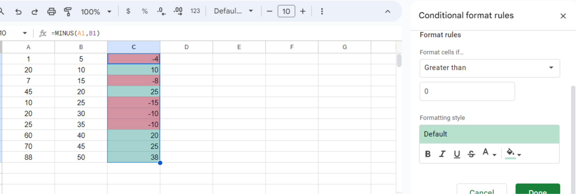
- Use the MINUS function: Follow the steps in method 2 to show the differences between the two columns.
- Select the Third Column: Highlight the entire third column (e.g., column C).
- Applying Conditional Formatting: Head to the top menu and click on "Format," then choose "Conditional formatting."
- Set Up the Rules: In the conditional formatting pane, select "Format cells if," and choose "Less than" or "Greater than," depending on your preference. Then, enter "0" in the next field.
- Choose a Format: Click on the paint bucket icon to select the formatting style you want for cells where the condition is met. You can tweak font colors, and backgrounds, or add other formatting options to make the differences stand out.
Now, Google Sheets will visually highlight cells in column C where the value is less than or greater than zero, indicating the differences between the two columns.
In conclusion, mastering the art of finding the difference between two columns in Google Sheets is a fundamental skill that can unlock insights within your data. Whether you're crunching numbers to compare sales figures, monitoring inventory fluctuations, or scrutinizing survey responses, the ability to calculate these differences is a valuable skill to have.

