How To Strikethrough in Excel: 8 Ways + Examples
Most would imagine that adding a strikethrough in Excel would be as simple as it is in Word - just a button click. However, while Excel is excellent for manipulating numbers, some processes can be convoluted. This is one of them! No need to worry; these step-by-step instructions have you covered.
What Is The Strikethrough Format?
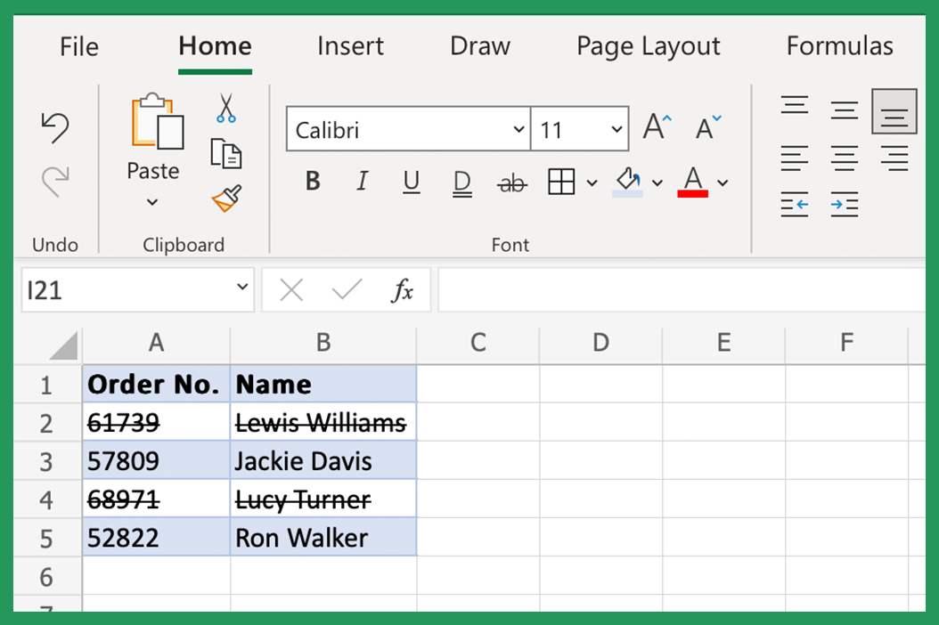
The strikethrough format is a character formatting option that is used to apply a line through the middle of the selected text. Strikethrough can be useful for showing edits or deletions in a document without permanently altering the original text. When you apply strikethrough to text, the text is not deleted; it remains in the cell.
Why Use Strikethrough Excel Formatting Buttons
The strikethrough function is useful for drawing attention to changes or edits. Strikethrough can also be used as a way of indicating that something is no longer relevant. For example, once you have the completed tasks, you can add strikethrough to show that it's done. You can do it easily the the use of other formatting buttons.
8 Ways to Add Strikethrough Formatting in Excel
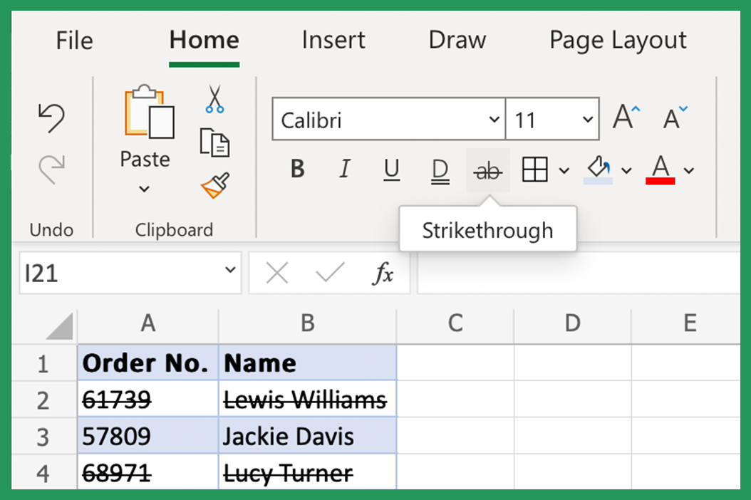
Wondering how to apply strikethrough format processes in your workbook? There are a few different ways to add strikethrough in Excel. The most straightforward way is to use the Font group on the Home tab. Then, simply select the data you want to strikethrough and click on the Strikethrough button (it looks like an ABC with a line through it).
Strikethrough Text Keyboard Shortcut
The quick keyboard shortcut for creating a strikethrough is Alt + H + S on windows or COMMAND + SHIFT + X on mac.
Using Format Cells Dialog Box to Add a Strikethrough
You can also use the Format Cells box to add strikethrough in Excel. Simply select the text you want to strikethrough, right-click and choose Format Cells. Then, check the Strikethrough box in the Font tab and click OK.
Using The Strikethrough Button
Another way to strikethrough in Excel is to apply the Strikethrough button on the Font group of the Excel ribbon. First, select the text you want to apply it to, click on the Strikethrough button (it looks like an ABC with a line through it), and then click away from the text to deselect it.
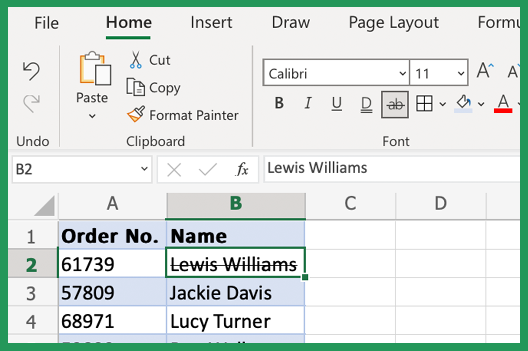
Apply Strikethrough to Multiple Texts in Excel
If you want to strikethrough multiple texts simultaneously, simply hold down the Ctrl key and select each item you wish to strikethrough. Then, apply it by clicking the button as before.
Using Excel's Conditional Formatting Feature
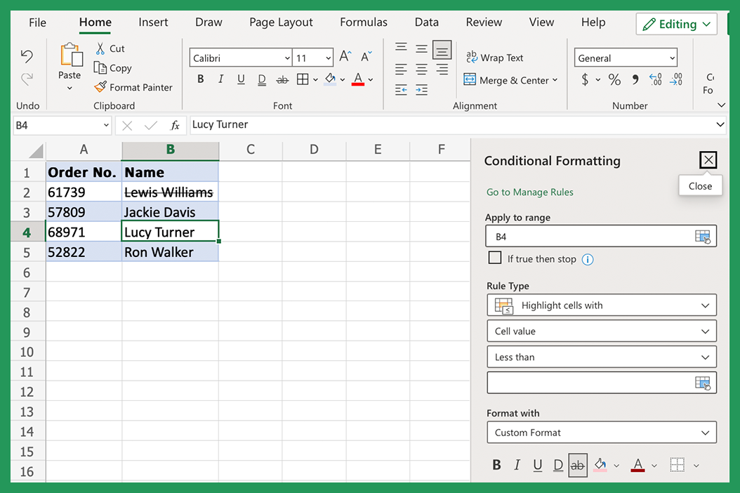
You can also use Excel's conditional formatting feature to strikethrough cells that meet certain criteria. For example, you could strikethrough all cells that contain a value less than 100.
To do this, select the cells you want to check, then click on Home and go to Conditional Formatting > Highlight Cell Rules > Less Than. In the box that appears, enter 100 and choose strikethrough from the drop-down menu next to Format cell. Finally, click OK to apply it.
Ctrl Keyboard Shortcut to Strikethrough Text in Excel
Finally, you can use a keyboard shortcut to strikethrough your text in Microsoft Excel. To do this, select the text you want to strikethrough and click Ctrl+Shift+X on your keyboard. This will instantly strikethrough the selected data. Now you can easily apply strikethrough format commands in Excel.
Adding a Strikethrough using a Macro
If you need to apply the Excel strikethrough formatting often, you can create a macro to do it for you. This way, all you need to do is press a button (or keyboard shortcut), and the strikethrough will be applied automatically.
A macro is a set of instructions that can be executed automatically. In Excel, macros are written in Visual Basic for Applications (VBA). VBA code is a programming language designed specifically for use with Microsoft Office applications.
You can use macros to automate repetitive tasks, or to perform complex tasks that would be difficult or impossible to do manually.
To create a macro, open the Visual Basic Editor by pressing Alt+F11 on your keyboard. Then, in the editor, mouse click Insert > Module. This will insert a new module into your workbook.
In the module, enter the following code:
Sub ApplyStrikethrough()
Selection.Font.Strikethrough = True
End Sub
Now, whenever you want to strikethrough content, just select it and press the play button in the top toolbar (or press F to run the macro).
How to Strikethrough Text using a Mac
A simple way to strikethrough text for Mac users is by using the following Strikethrough command keyboard shortcut: ⌘ + SHIFT + X
Like on Windows operating systems, you can also use the Font dialog box or the Format Cells dialog box to strikethrough text in Excel.
Format Strikethrough using the Font Box or Format Cells Box
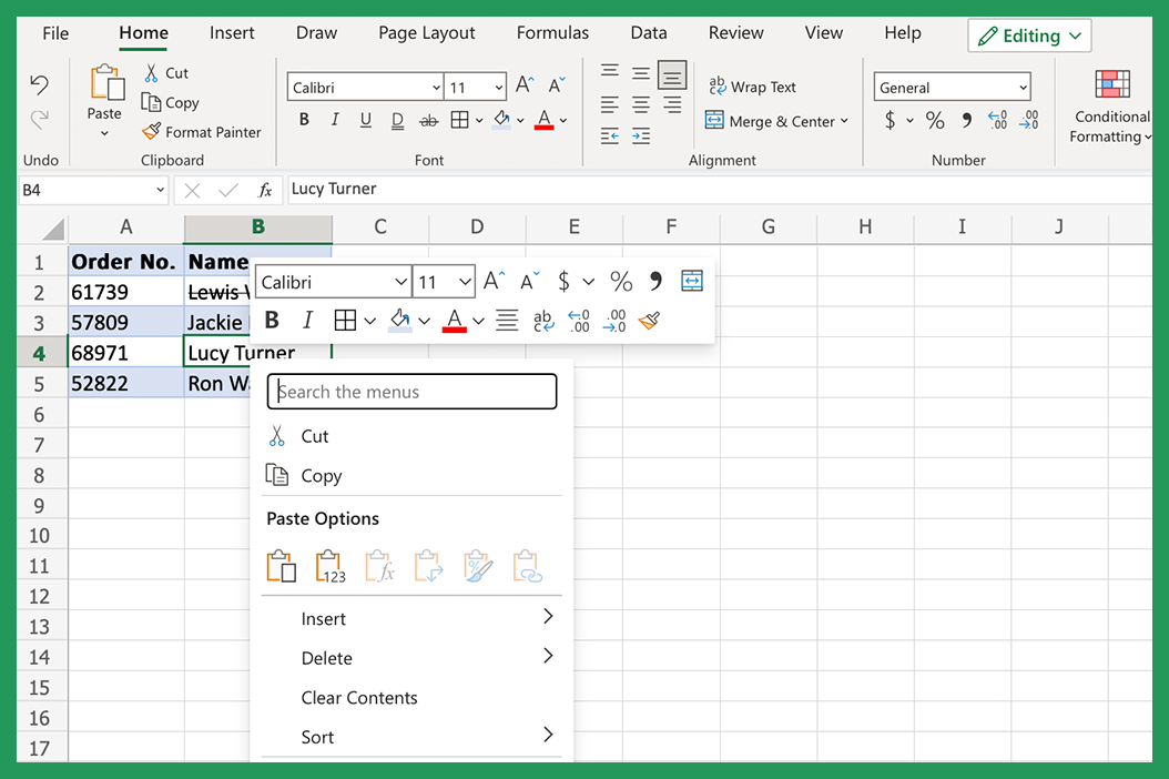
To strikethrough content in Excel for Mac using the popup menu:
- Select the cells with the text you want to strikethrough.
- On the Home tab, click the Font Dialog box launcher.
- In the same tab, select the option to strikethrough in the Effects section.
- Click OK.
How to add a Strikethrough Format to the Quick Access Toolbar in Excel
To add a Strikethrough format to the Quick Access Toolbar in Excel, do the following:
- On the Home tab, click the Strikethrough button.
- Click the Customize Quick Access Toolbar button.
- In the Customize Quick Access Toolbar popup box, select Strikethrough in the Commands list.
- Click Add.
- Click OK.
Removing the Format in the Quick Access Toolbar
You can follow the steps below to remove the format using the Quick Access Toolbar button.
- On the Home tab, click the button to add Strikethrough.
- Click the Customize Quick Access Toolbar button.
- In the Customize Quick Access Toolbar box, select Strikethrough in the Commands list.
- Click Remove.
- Click OK.
Once you have the Excel strikethrough button added to your Quick Access Toolbar, you can use it right away.
Guide to Removing Strikethrough Format Cells in Excel
How to Remove Strikethrough Formatting
To remove the strikethrough from your text, use the following steps, and refer to our example above:
- Select the cells with the text you want to strikethrough.
- On the Home tab, click the Font box launcher.
- In the tab, clear the Strikethrough checkbox in the Effects section.
- Click OK.
How to Remove Strikethrough using the Font Dialog Box
You can also remove the strikethrough by using the Font dialog box shortcut commands below:
- Select the cells with the strikethrough texts you want to remove.
- Press Ctrl+D on your keyboard. This shortcut opens the Font tab in the Format Cells popup box.
- In the Effects section, clear the Strikethrough check box.
- Click the OK button.
How To Apply & Remove Partial Strikethrough Format in a Cell
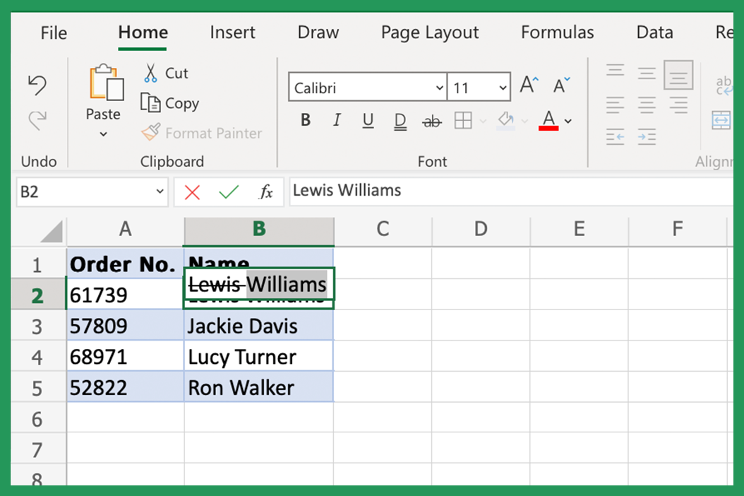
Applying a partial strikethrough is useful when you want to indicate that someone has changed their mind about something, or if something is partially no longer relevant, but you still want to keep it in the selected cell for reference. Adding strikethroughs partially is actually fairly simple to do.
To apply a partial strikethrough format:
- Select the cell contents you want to add a strikethrough to.
- Press Ctrl+D on your keyboard. This shortcut opens the Font tab in the Format Cells dialog menu.
- In the Effects section, click Strikethrough check box.
- Click the OK button to add the new formatting to the cell.
To remove the partial strikethrough format, apply the following steps:
- Select the strikethrough string within the cell.
- Press Ctrl+D on your keyboard. This shortcut opens the Font tab in the Format Cells dialog box.
- In the Effects section, clear the Strikethrough check box.
- Click OK.
Excel Tips & Tricks for Beginners
One of the best things about Microsoft Excel is that it is extremely versatile. You can use it for a wide range of tasks, from organizing your finances to tracking your fitness progress. And, if you know the right tips and tricks, you can make your life a whole lot easier.
If you're new to Excel, or simply want to brush up on your Excel skills, then this extra little guide is for you. We've put together our top Excel tips and tricks, so you can make the most of this powerful software.
One of the most basic but essential things you can do in Excel is format cells. This means changing the way they look, such as the font, color, or size. You might also want to apply a border, use a strikethrough format, or background color or add a cell comment.
Formatting can make your content much easier to read and understand. It can also help you to highlight important information, such as negative values in red or sales figures in green.
To format cells in Excel, first select the content you want to format. Then, click the Home tab on the ribbon and look for the Font section. Here, you can change the text type, size, color, and style.
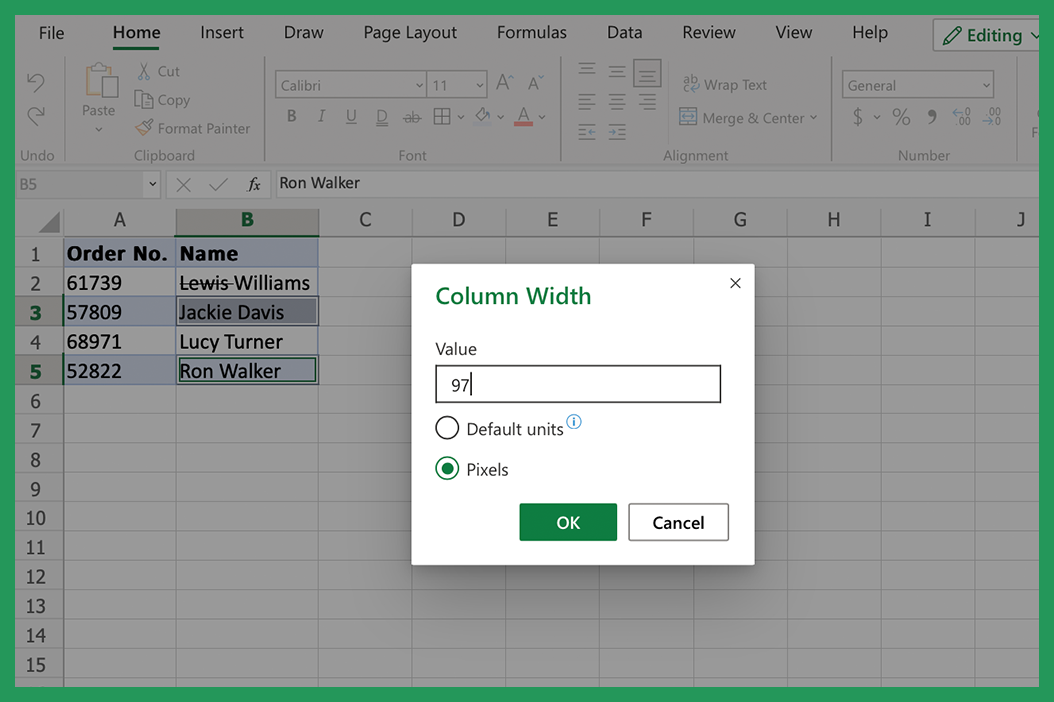
You can also use the Format Cells dialog box to apply more advanced formatting options. To open this dialog box, select the text you want to format and press Ctrl + 1 on your keyboard.
In the Format Cells dialog box, you can change the number format, alignment, text color, and other options. You can also add a border or background color, or add a cell comment.
When you're finished formatting, click OK to close the dialog box. Your changes will be applied to the selected cells.
You can also format cells using the conditional formatting feature in Excel. With conditional formatting, you can apply formatting automatically based on the value in a cell.
For example, you could use conditional formatting to highlight cells that are greater than or equal to a certain value. Or, you could use it to apply different colors to cells based on their values.
Applying Strikethrough Formatting in Excel
The Strikethrough option in text formatting allows you to draw a line through your text. It's often used to indicate that something is no longer relevant or to show that something has been completed.
In Excel, you can apply strikethrough formatting to cells in a worksheet. If you've got this far, it means you already know how to do this!
Quick Summary & Tips for Excel Newbies
We know excel is fantastic for manipulating numbers. However, it can be daunting for newbies due to the sheer mass of formats and processes available. Below, we've summarised the above points into more manageable snippets to revert back to. We've also included a few extra tips you might find useful.
- To quickly select all cells with Strikethrough formatting, use this keyboard shortcut: CTRL + SHIFT + F. This will open the Find and Replace dialog box with the Strikethrough option already selected in the Format box.
- To remove Strikethrough formatting from cells, select the cells and press CTRL + SHIFT + F to open the Find and Replace dialog box. Then, in the Format cells section, click strikethrough and then the Clear Formatting button.
- You can also use the shortcut ALT + H + F + S to strikethrough cells in Excel.
Conclusion
There you have it! You now have access to eight different ways to apply strikethrough formatting in Excel. We hope you found the right solution or answer for you. Adding strikethrough formats really is that simple. With so many ways to do it, you can't go wrong. This formatting command is a great way to make your spreadsheet more organized and easier to manage.
You can use the quick methods mentioned in this article to make your Excel worksheets more organized and easier to read by adding strikethrough formats. Anyone who works with Excel knows it can get complicated and overwhelming if you don't manage the spreadsheet and make use of the many formatting options available to you. The more commands you know, the better.
Do you have any other tips for using strikethrough in Excel? Share them with us via our contact page!

